|
||||||
|
JPEG Compression
(taken from CMPT 365 homepage at SFU)Motivations:
- Uncompressed video and audio data are huge. In HDTV, the bit rate easily exceeds 1 Gbps. --> big problems for storage and network communications.
-
The compression ratio of lossless methods (e.g., Huffman, Arithmetic, LZW) is not high enough for image and video compression, especially when distribution of pixel values is relatively flat.
- Spatial Redundancy Removal -- Intraframe coding (JPEG)
- Spatial and temporal Redundancy Removal -- Intraframe and Interframe coding (H.261, MPEG)
1. What is JPEG?
- "Joint Photographic Expert Group". Voted as international standard in 1992.
- Works with color and grayscale images, e.g., satellite, medical, ...
2. JPEG overview
- Encoding
- Decoding -- Reverse the order
3. Major Steps
- DCT (Discrete Cosine Transformation)
- Quantization
- Zigzag Scan
- DPCM on DC component
- RLE on AC Components
- Entropy Coding (i.e. Huffman Coding)
3a. Discrete Cosine Transform (DCT)
- Overview:
- Definition (8 point DCT):
Question: What is F[0,0]? -- define DC and AC components.
- The 64 (8 x 8) DCT basis functions
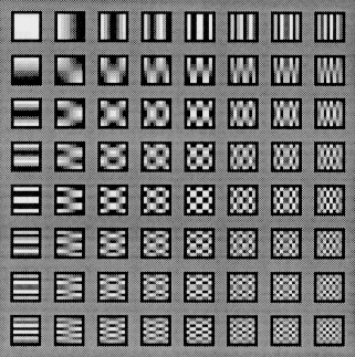
- Why DCT not FFT?
DCT is like FFT, but can approximate lines well with few coeff.
- Computing the DCT
- Factoring reduces problem to a series of 1D DCTs:
- Most software implementations use fixed point arithmetic. Some fast implementations approximate coefficients so all multiplies are shifts and adds.
- World record is 11 multiplies and 29 adds. (C. Loeffler, A. Ligtenberg and G. Moschytz, "Practical Fast 1-D DCT Algorithms with 11 Multiplications", Proc. Int'l. Conf. on Acoustics, Speech, and Signal Processing 1989 (ICASSP `89), pp. 988-991)
- Factoring reduces problem to a series of 1D DCTs:
3b. Quantization
- Why? -- To throw out bits
- Example: 101101 = 45 (6 bits).
Truncate to 4 bits: 1011 = 11.
Truncate to 3 bits: 101 = 5.
Uniform quantization
- Divide by constant N and round result (N = 4 or 8 in examples above).
- Non powers-of-two gives fine control (e.g., N = 6 loses 2.5 bits)
Quantization Tables
- In JPEG, each F[u,v] is divided by a constant q(u,v).
- Table of q(u,v) is called quantization table.
----------------------------------

16  11  10  16  24   40   51   61

12  12  14  19  26   58   60   55

14  13  16  24  40   57   69   56

14  17  22  29  51   87   80   62

18  22  37  56  68   109  103  77

24  35  55  64  81   104  113  92

49  64  78  87  103  121  120  101

72  92  95  98  112  100  103  99

----------------------------------
- Eye is most sensitive to low frequencies (upper left corner), less sensitive to high frequencies (lower right corner)
- Standard defines 2 default quantization tables, one for luminance (above), one for chrominance.
- Q: How would changing the numbers affect the picture (e.g., if I doubled
them all)?
Quality factor in most implementations is the scaling factor for default quantization tables.
- Custom quantization tables can be put in image/scan header.
3c. Zig-zag Scan
- Why? -- to group low frequency coefficients in top of vector.
- Maps 8 x 8 to a 1 x 64 vector
3d. Differential Pulse Code Modulation (DPCM) on DC component
- DC component is large and varied, but often close to previous value (like lossless JPEG).
- Encode the difference from previous 8x8 blocks -- DPCM. Only send the DC value of the first block and then the subsequent differences.
3e. Run Length Encode (RLE) on AC components
- 1x64 vector has lots of zeros in it
- Encode as (skip, value) pairs, where skip is the number of zeros and value is the next non-zero component.
- Send (0,0) as end-of-block sentinel value.
3f. Entropy Coding
- Categorize DC values into SSS (number of bits needed to represent) and actual
bits.
-------------------- Value SSS 0 0 -1,1 1 -3,-2,2,3 2 -7..-4,4..7 3 -------------------- - Example: if DC value is 4, 3 bits are needed.
Send off SSS as Huffman symbol, followed by actual 3 bits.
- For AC components (skip, value), encode the composite symbol (skip,SSS) using the Huffman coding.
- Huffman Tables can be custom (sent in header) or default.
- About Huffman Coding
4. Overview of the JPEG bitstream
- A "Frame" is a picture, a "scan" is a pass through the pixels (e.g., the red component), a "segment" is a group of blocks, a "block" is an 8x8 group of pixels.
- Frame header:
sample precision
(width, height) of image
number of components
unique ID (for each component)
horizontal/vertical sampling factors (for each component)
quantization table to use (for each component) - Scan header
Number of components in scan
component ID (for each component)
Huffman table for each component (for each component) - Misc. (can occur between headers)
Quantization tables
Huffman Tables
Arithmetic Coding Tables
Comments
Application Data
5. Various JPEG Modes
- Baseline/Sequential -- the one that we described in detail
- Lossless
- Progressive
- Hierarchical
- "Motion JPEG" -- Baseline JPEG applied to each image in a video.
- Lossless Mode
- A special case of the JPEG where indeed there is no loss
- Take difference from previous pixels (not blocks as in the Baseline
mode) as a "predictor".
Predictor uses linear combination of previously encoded neighbors.
It can be one of seven different predictor based on pixels neighbors
- Since it uses only previously encoded neighbors, first row always uses P2, first column always uses P1.
- Effect of Predictor (test with 20 images)
Note: "2D" predictors (4-7) always do better than "1D" predictors.
Comparison with Other Lossless Compression Programs (compression ratio):
----------------------------------------------------------------- Compression Program Compression Ratio Lena football F-18 flowers ----------------------------------------------------------------- lossless JPEG 1.45 1.54 2.29 1.26 optimal lossless JPEG 1.49 1.67 2.71 1.33 compress (LZW) 0.86 1.24 2.21 0.87 gzip (Lempel-Ziv) 1.08 1.36 3.10 1.05 gzip -9 (optimal Lempel-Ziv) 1.08 1.36 3.13 1.05 pack (Huffman coding) 1.02 1.12 1.19 1.00 ----------------------------------------------------------------- - A special case of the JPEG where indeed there is no loss
- Progressive Mode
- Goal: display low quality image and successively improve.
- Two ways to successively improve image:
- Spectral selection: Send DC component, then first few AC, some more AC, etc.
- Successive approximation: send DCT coefficients MSB (most significant bit) to LSB (least significant bit).
- Hierarchical Mode
A Three-level Hierarchical JPEG Encoder
(From V. Bhaskaran and K. Konstantinides, "Image and Video Compression Standards: Algorithms and Architectures", Kluwer Academic Publishers, 1995.)
- Down-sample by factors of 2 in each direction.
Example: map 640x480 to 320x240
- Code smaller image using another method (Progressive, Baseline, or Lossless).
- Decode and up-sample encoded image
- Encode difference between the up-sampled and the original using Progressive, Baseline, or Lossless.
- Can be repeated multiple times.
- Good for viewing high resolution image on low resolution display.
- Down-sample by factors of 2 in each direction.
- JPEG-2
- Big change was to use adaptive quantization