|
||||||
|
Scale-space representation: Definition and basic ideas
(taken from http://www.nada.kth.se/~tony/cern-review/cern-html/node2.html)
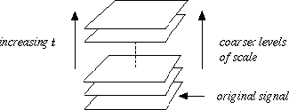
Figure 1: A multi-scale representation of a
signal is an ordered set of derived signals intended to represent the original
signal at different levels of scale.
Scale-space theory is a framework for early visual operations, which has been
developed by the computer vision community (in particular by Witkin , Koenderink
, Yuille and Poggio, Lindeberg and Florack ) to handle the above-mentioned
multi-scale nature of image data. A main argument behind its construction is
that if no prior information is available about what are the appropriate scales
for a given data set, then the only reasonable approach for an uncommitted
vision system is to represent the input data at multiple scales. This means that
the original signal should be embedded into a one-parameter family of derived
signals, in which fine-scale structures are successively suppressed (see
figure 1). How should such an idea be carried out in practice? A crucial
requirement is that structures at coarse scales in the multi-scale
representation should constitute simplifications of corresponding structures at
finer scales--they should not be accidental phenomena created by the method for
suppressing fine-scale structures. This idea has been formalized in a variety of
ways by different authors. A noteworthy coincidence is that similar conclusions
can be obtained from several different starting points. A main result is that if
rather general conditions are imposed on the types of computations that are to
be performed, then convolution by the Gaussian kernel and its derivatives is
singled out as a canonical class of smoothing transformations. The requirements
(scale-space axioms) that specify the uniqueness are essentially linearity and
spatial shift invariance, combined with different ways of formalizing the notion
that new structures should not be created in the transformation from fine to
coarse scales. In summary, for any N-dimensional signal ![]() ,
its scale-space representation
,
its scale-space representation ![]() is defined by
is defined by ![]()
where ![]() denotes the Gaussian kernel
denotes the Gaussian kernel
![]()
and the variance t
of this kernel is referred to as the scale parameter. Equivalently, the
scale-space family can be obtained as the solution to the (linear) diffusion
equation ![]()
with initial condition ![]() .
Then, based on this representation, scale-space derivatives at any
scale t are defined by
.
Then, based on this representation, scale-space derivatives at any
scale t are defined by ![]()

Figure 2: (a) The main idea of a scale-space
representation is to generate a one-parameter family of derived signals in which
the fine-scale information is successively suppressed. This figure shows a
signal which has been successively smoothed by convolution with Gaussian kernels
of increasing width. (b) Since new zero-crossings cannot be created by the
diffusion equation in the one-dimensional case, the trajectories of
zero-crossings in scale-space (here, zero-crossings of the second derivative)
form paths across scales that are never closed from below.

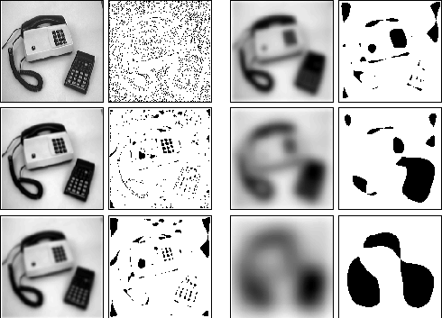
Figure 3: Different levels in the scale-space
representation of a two-dimensional image at scale levels t = 0, 2, 8,
32, 128 and 512 together with grey-level blobs indicating local minima at each
scale.
Figure 2(a) shows the result of applying Gaussian smoothing to a one-dimensional signal in this way. Notice how this successive smoothing captures the intuitive notion of fine-scale information being suppressed, and the signals becoming successively smoother. Figure 3 gives a corresponding example for a two-dimensional image. Here, to emphasize the local variations in the grey-level landscape, local minima in the grey-level images at each scale have been indicated by dark blobs (with spatial extent determined from a certain watershed analogy, which essentially describes how large a region associated with a local minimum can be filled with water, without water flooding over to regions associated with other local minima). As can be seen, mainly small blobs due to noise and texture are detected at fine scales. After a small amount of smoothing, the buttons on the keyboard manifest themselves as distinct minima, whereas at even coarser scales they merge to one unit (the keyboard). Also other dominant dark image structures (such as the calculator, the cord and the receiver) appear as single blobs at coarser scales. This example gives one illustration of the types of hierarchical shape decompositions that can be obtained by varying the scale parameter in the scale-space representation. The relations between image structures at different scales induced in this way is referred to as deep structure .
Interestingly, the results of this computationally motivated analysis are
in qualitative agreement with the results of biological evolution.
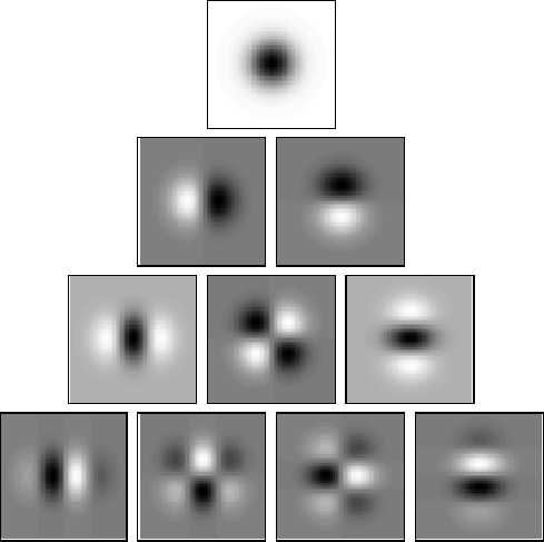
Neurophysiological studies by Young have shown that there are receptive field
profiles in the mammalian retina and visual cortex, which can be well modelled
by superpositions of Gaussian derivatives. 
Figure 4: Gaussian derivative kernels up to order four the two-dimensional
case.
